Reinforcement Learning Expanded Introduction
Reinforcement Learning on a more serious note…
Reinforcement learning (RL) is a framework for learning optimal behavior through trial-and-error interaction with an environment. Unlike supervised learning (where we have correct answers) or unsupervised learning (where we find patterns), RL learns from rewards and penalties.
When learning to drive: You don’t get a manual with every possible scenario - instead, you learn by trying actions (steering, braking) and experiencing consequences (smooth ride, honking horns, accidents). Over time, you develop a driving policy that maximizes good outcomes.
The RL Framework: Agent-Environment Interaction
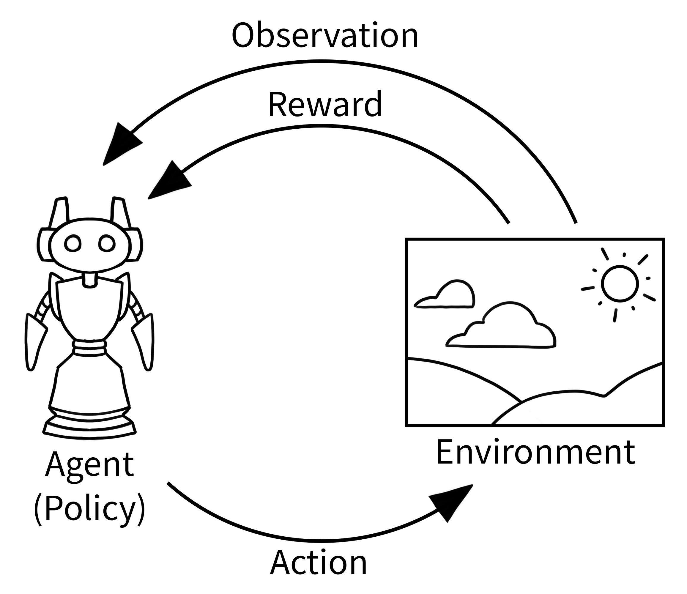
Figure 1: The fundamental RL loop where an agent takes actions in an environment and receives observations and rewards
Core Components
- Agent: The learner/decision-maker (you, the driver)
- Environment: Everything outside the agent (road, other cars, traffic laws)
- State (s_t): The true state of the environment at time t (positions of all cars, traffic light status)
- Observation (o_t): What the agent actually perceives (what you see through your windshield)
- Action (a_t): Choice made by the agent (turn left, brake, accelerate)
- Reward (r_t): Feedback signal from environment (+1 for reaching destination, -100 for accident)
The Markov Property: Why States Matter
The Markov property states that the future state depends only on the current state, not on the sequence of events that led to the current state. This is a key assumption that makes the problem tractable (manageable).
P(s_{t+1} | s_t, a_t, s_{t-1}, a_{t-1}, ...) = P(s_{t+1} | s_t, a_t)
Explanation: The equation states that the probability of transitioning to state s_{t+1} depends only on the current state s_t and current action a_t, not on any previous states or actions. The left side shows the full history-dependent probability, while the right side shows it reduces to just the current state-action pair.
Driving analogy: To predict what happens next, you only need to know current positions and speeds, not how cars got there. This makes the problem tractable, otherwise we’d need infinite memory.
Policies and Value Functions
Policy (\pi)
A policy maps states to actions: \pi(a|s) = P(A_t = a | S_t = s)
- Deterministic policy: a = \pi(s) (always take same action in same state)
- Stochastic policy: \pi(a|s) (probability distribution over actions)
Value Functions: Measuring Long-term Success
The state value function measures expected cumulative discounted reward. V^\pi(s) quantifies the expected total discounted reward an agent will accumulate starting from state s and following policy \pi forever. The discount factor \gamma exponentially reduces the weight of future rewards - a reward k steps in the future gets weighted by \gamma^k. The discount factor is a hyperparameter that controls how much we value future rewards compared to immediate rewards.
The equation defines how we measure the “goodness” of being in a particular state under a specific policy.
Example: When evaluating a job offer, the “value” of accepting the job isn’t just your first paycheck - it’s all future paychecks combined, but you care less about paychecks 10 years from now than next month’s paycheck. The discount factor is like your personal “impatience rate.”
V^\pi(s) = \mathbb{E}_\pi\left[\sum_{k=0}^{\infty} \gamma^k R_{t+k+1} \mid S_t = s\right]
Where:
- \gamma \in [0,1] is the discount factor (future rewards matter less)
- k is the time offset - it represents how many time steps into the future we’re looking from the current time t.
- R_{t+k+1} is the reward at time t+k+1
Why discounting?
- Uncertainty increases with time
- Immediate rewards often preferred (bird in hand…)
- Mathematical convenience (prevents infinite sums)
Action-Value Function (Q-function)
This tells us: “How good is taking action a in state s, then following policy \pi?”
The action-value function (Q-function) measures the expected cumulative discounted reward from taking a specific action in a specific state, then following the policy thereafter.
Q^π(s,a) quantifies the total expected return when you take action a in state s, then follow policy \pi for all subsequent decisions. It’s conditioned on both the initial state AND the initial action, unlike the state value function which only conditions on the state.
Evaluating a chess move: The Q-function answers: “If I make this specific move right now, then play optimally (according to my strategy) for the rest of the game, what’s my expected final score?” It’s not just asking “how good is this position?” but “how good is this specific move from this position?”
Q^\pi(s,a) = \mathbb{E}_\pi\left[\sum_{k=0}^{\infty} \gamma^k R_{t+k+1} \mid S_t = s, A_t = a\right]
The Optimal Policy
We seek the policy that maximizes expected return:
\pi^* = \arg\max_\pi \mathbb{E}_{s_0 \sim \rho}[V^\pi(s_0)]
Where: - \rho is the distribution over initial states. - s_0 is the initial state. - \mathbb{E}_{s_0 \sim \rho} means “the expected value of the initial state under the distribution \rho”. - \pi is the policy. - V^\pi(s_0) is the value of the initial state under policy \pi. - \arg\max_\pi means “the policy that maximizes the expected return” (point us to the best (max/optimal) policy).
Bellman Optimality Equation: V^*(s) = \max_a \sum_{s'} P(s'|s,a)[R(s,a,s') + \gamma V^*(s')]
This recursive relationship is the foundation of many RL algorithms.
Exploration vs. Exploitation: The Central Dilemma

Figure 2: The exploration-exploitation dilemma - balancing trying new actions vs. using known good actions
The dilemma: Should you:
- Exploit: Use current knowledge to maximize immediate reward
- Explore: Try new actions to potentially find better options
Restaurant analogy: You know one good restaurant (exploit) but there might be amazing places you haven’t tried (explore). Pure exploitation means you might miss the best restaurant in town. Pure exploration means constantly eating at mediocre new places.
Epsilon-Greedy Strategy
- With probability 1-\epsilon: choose best known action (exploit)
- With probability \epsilon: choose random action (explore)
Multi-Armed Bandits: RL Without States
Bandits are a special case where: - No state transitions (each action is independent) - No temporal dependencies - Pure exploration vs. exploitation problem

Figure 3: Multi-armed bandit - multiple slot machines with unknown payout rates
Key difference from full RL: In bandits, your choice of slot machine doesn’t affect which machines are available next. In full RL, your actions change the state and future options.
Upper Confidence Bound (UCB)
Choose action that maximizes: \hat{\mu}_a + \sqrt{\frac{2\ln t}{n_a}}
Where: - \hat{\mu}_a = estimated mean reward for action a - n_a = number of times action a was chosen - t = total number of rounds
The square root term represents uncertainty - actions tried less often get exploration bonus.
Learning Approaches
Model-Based vs. Model-Free
Model-Based: Learn environment dynamics P(s'|s,a) and R(s,a), then plan - Like studying road maps before driving - Can be sample efficient but computationally expensive
Model-Free: Learn policy/values directly from experience - Like learning to drive just by practicing - Less sample efficient but often more practical
Temporal Difference Learning
Key insight: We don’t need to wait until episode ends to learn!
TD Error: \delta_t = r_{t+1} + \gamma V(s_{t+1}) - V(s_t)
Q-Learning Update: Q(s_t, a_t) \leftarrow Q(s_t, a_t) + \alpha[r_{t+1} + \gamma \max_a Q(s_{t+1}, a) - Q(s_t, a_t)]
This lets us learn from every single step, not just complete episodes.
Common Pitfalls and Misconceptions
- State vs. Observation confusion: The agent rarely sees the full state
- Assuming deterministic environments: Most real environments have randomness
- Ignoring exploration: Greedy policies often get stuck in local optima
- Reward hacking: Agents optimize exactly what you specify, not what you intend
Real-World Applications
- Autonomous driving: States = traffic situations, Actions = steering/speed control
- Game playing: AlphaGo, StarCraft II agents
- Recommendation systems: States = user preferences, Actions = what to recommend
- Resource allocation: Cloud computing, power grid management
- Robotics: Learning motor skills, manipulation
Key Takeaways
- RL solves sequential decision problems through trial-and-error
- The Markov property makes problems tractable
- Balancing exploration and exploitation is crucial
- Value functions capture long-term consequences of actions
- We can learn incrementally without complete episodes
The power of RL lies in learning optimal behavior without being explicitly told what to do - just by experiencing consequences and optimizing for long-term success.